About

This article is a summary/conversion of information into a blog for a research paper titled, "State-and-Transition Simulation Models: A Framework For Forecasting Landscape Change", written by Colin J. Daniel, Leonardo Frid, Benjamin M. Sleeter, and Marie-Josee Fortin.

You can find a link to the paper itself here.

Introductions

Simulation models are valuable in understanding and analyzing insights into the dynamics of landscapes composed of nature and human influence.

Many simulation models have been developed since the 1970s, such as that of landscape vegetation models, developed principally by ecologists. These models focused on landscape-scale changes, vegetation, ecological drivers due to climate, biophysical conditions. However, we have so far not been able to generalize these models to various systems.

More-over, there is an interesting category of LULC change models. land-user/land-cover abbreviated is LULC. Here, the focus is on the effects of human-driven processes on the LULC change.

These models often share landscape dynamics, sharing common features, many of which are important in generalized landscape modelling framework. The resulting research work has resulted in development of landscape vegetation models for a range of ecological systems.

In context with the paper, this is referred to as "State-And-Transition Simulation Model" (STSM). It can be characterized as,

1. Space is represented as a set of discrete spatial units
2. Time is represented in discrete steps
3. The change over time in the discrete state of each spatial unit is represented as a stochastic process
4. Time-in-homogeneous rates of change between states are expressed as probabilities

There is somewhat of a similarity between STSMs and Markov Chains, but the differences are strikingly sufficient to treat each as differently. This can be said the same for "Cellular Automata Models" and STSMs

STSM Approach

Steps include,

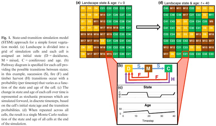
1. Dividing the landscape spatially into a set C of n simulation cells. Cells can be of any shape/size, commonly represented as a regular raster grid
2. In STSM, the change in state of each simulation cell over time as a discrete-time stochastic process {X_t : t >= 0}, WHERE State Space is a set S of 'r' discrete state types (X_t belongs to S), and 't' represents discrete timestamps

STSM Distinguishment

In landscape models, it is important to distinguish different types of transitions between states, which is not possible within Markov Chains.

In Markov, multiple factors of the simulated system are combined into a single transition probability between any two states in a Markov chain representation.

With STSM, a set U of m discrete transition types are defined for all cells, with a separate transition matrix P defined or each possible transition type k belongs to U. The nonzero entries across all P are referred to as transition pathways. Separate transition matrix for succession, wildfire, and timber harvest exist.

STSM vs Markov Chain

To accommodate multiple requirements for multiple transition types in an STSM, within each time-step the transition matrices, P, applied sequentially for each transition type k belongs to U in order to update the state of each cell between timestamps.

Another change between STSMs and Markov Chains is that with STSMs 'counters' can be defined as additional state variables for each cell in a simulation and then incremented by one for every time-step.

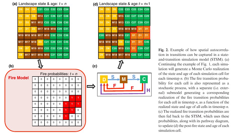
Age And Time-Since-Transition

For each cell, there are time-state-transition (TST) used to track the age. Where TST refers to the number of time-steps that have elapsed since one or more transition types last occurred.

Formulating a stochastic process this way, however, results in an unmanageable large state space for even the simplest models. STSMs instead track each counter (in addition to the state type X_t), as a separate discrete-time stochastic process.

This consists of a grid that is updated every timestep according to the following rules,

1. If a transition occurs for a cell, then a corresponding probability distribution is used to determine the fate of the cell's age; these probability distribution for the change in age can vary as a function of the state of the cell (i.e., its state type, age and TST) and the type of transition
2. If no transition occurs for the cell, then the age of the cell is incremented by 1. The TST is tracked in a similar way and repeated for each transition type

Transition Targets

Another limitation of Markov Chains is that transitions between states must always be characterized in terms of a probability of occurrence. Some transitions are expected to be more management-oriented, however, as they involve an expression for a target for the area to be transitioned over time, rather than a probability.

With STSMs, transitions can be characterized using either probabilities or target areas, where targets are dynamically converted into transition probabilities during the simulation. This can be calculated if one knows the full state of landscape targets to be specified for other derived variables.

Spatial And Temporal Heterogeneity

State variables in STSMs are random variables, there is some inherent variability in when and where transitions occur in any one realization of a model.

In addition to temporal variability, the transition probabilities in STSMs can also vary spatially - it is possible to vary the transition probability for every cell and time-step the landscape.

To accommodate this requirement, the transition probabilities in an STSM can also be expressed as random variables for each cell and time-step; as a result, it is ultimately possible to generate any spatial and temporal pattern of transitions on the landscape.

Simplification

To simplify the representation of spatial and temporal variation in transition probabilities, a two-step process is often used with STSMs.

First, a base probability for each transition type is defined as random variable. Transition multipliers are then specified in order to scale the base probabilities over space and time. These multipliers are defined as a stochastic process for each transition type and cell, the distribution of which can also be space and time in-homogenous.

To reproduce historical wildfire patterns in an STSM, the base wildfire probability is often estimated as a function of the long-term mean fire cycle, while the relative frequency distribution of area burned each year can be used to estimate the multipliers.

Software

Key aspects of the modelling framework will be a supporting piece of software to help with developing particularly larger and more complicated models. For this purpose, a software product called ST-Sim, released in 2013, was created to support the development of STSMs.

ST-Sim is raster-based. This allows it to handle simulations across larger (i.e., 10^6 cells). It also allows users to integrate external modules (R, Python).

Case Study Example - Hawai'i

This case study deals with presenting a simple model of the dynamics of LULC for the state of Hawai'i (USA). The purpose of this modelling effort is to explore the interactions between possible future changes in LULC.

This combined with projected shifts in plant communities due to climate change.

It is important to note that the description of the model and presentation of results here is purposefully brief, considering only a single "business-as-usual" future scenario, in order to remain focused upon the relationship between various features of the model and the STSM method presented above, rather than the broader context for the model's development and the interpretation of results.

State Variables And Scales

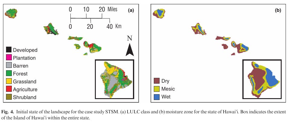
The spatial extent for this model is the terrestrial portion of the state of Hawai'i, covering 16,416 km^2. The landscape is divided spatially into simulation cells, each of which is 1x1 km in size. Simulations were run for 50 years with an annual time-step, using initial conditions corresponding to the year 2011; all simulations were repeated for 100 Monte Carlo realizations.

In STSMs, each cell in the simulation is characterized according to a suite of state variables, all of which are random, calculated for each simulation time-step.

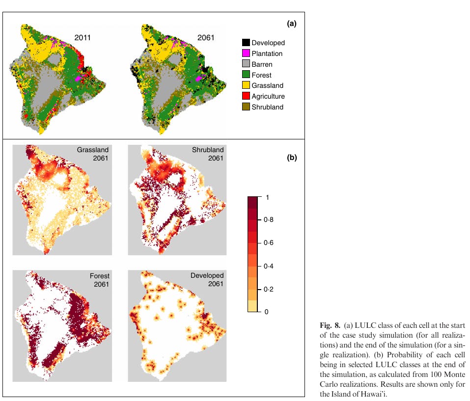
The first state variable is the state type of each cell: a total of 21 possible state types defined for this model, consisting of all unique combinations of seven LULC classes, crossed with three possible moisture zones.

The second state variable is that of age of cell (time-steps). The final state is the number of time-steps since the last time-steps since the last Transition (TST) for each cell, which for this model was only tracked for state types associated with the Grassland LULC class.

Model Formation

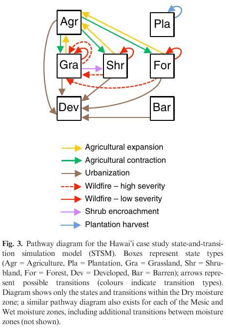
With all STSMs, a set of all the possible transition pathways between state types is defined.

The process represented by these transitions include expansion and contraction of agricultural lands, urbanization, wildfire, shrub encroachment into grassland, harvest of tree plantations, shift in moisture zones due to climate change.

Transitions due to agricultural expansion/contraction, urbanization are modeled using STSM transition targets. In order to represent the historical temporal variability in land-use change, the simulated annual transition areas are sampled for each year and Monte Carlo realization from a uniform distribution lifted to the corresponding historical land change data.

Based upon existing zoning maps, static transition multipliers were generated to,

1. Restrict agricultural expansion to areas zoned for agriculture
2. Prevent agricultural contraction from occurring in important agricultural areas
3. Prevent urbanization from areas zoned for conservation, and double the relative transition probability of urbanization in areas zoned as either urban or rural. In order to 'spread' transitions over time, transition multipliers are also generated (external model), for each cell, time-step and realization, such that,
   1. For agricultural expansion and urbanization, the relative transition probability increases linearly (from 0 to 1) as a function of the proportion of adjacent cells that are agriculture or developed
   2. For agricultural contraction, the relative transition probability increases linearly (from 0 to 1) as a function of the proportion of adjacent cells that are forest/shrubland/grassland.

Sub-Model

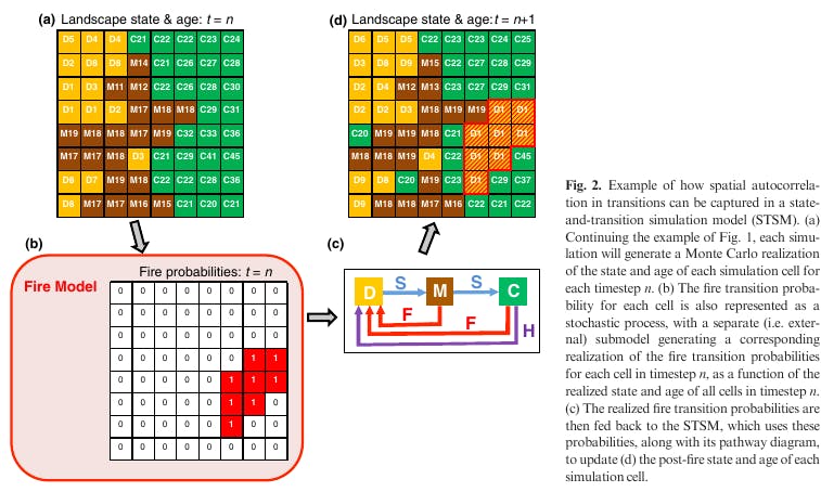
A separate wildfire sub-model is integrated into the STSM to determine which cells incur wildfire transitions for each simulated year and realization. This sub-model aims to reproduce the spatial and temporal pattern of historical wildfires.

The wildfire sub-model is integrated into the STSM to determine which cells incur wildfire transitions for each simulated year, and realization. This sub-model aims to reproduce the spatial and temporal pattern of historical wildfires.

The result of this submodel are then used to dynamically assign transition probabilities of 1 for those cells that transition each year and 0 for all other cells. The wildfire sub-model generates two sets of these transition probabilities for each time-step and realization, one for each of two classes (high and low) of fire severity.

Shrub Encroachment

Shrub encroachment is hypothesized to occur in the absence of regular fires - however, there is an uncertainty over how long this process will take.

Shrub Encroachment is represented as the following,

1. Transitions are restricted to cells in states associated with the Grassland LULC class where the time-since-fire is at least 10 years and the moisture zone is Dry or Mesic

2. At least one of the cell's eight neighbors must be in a state associated with the Shrubland LULC class

3. Annual transition probability is sampled from a uniform distribution for each realization, where the bounds of this distribution were set to 0.006 and 0.0327, corresponding to a cumulative transition probability of 0.95 from 10 to 500 and 50 years with fire, respectively.

Tree Plantations & Harvestation

Tree plantations in Hawai'i are generally harvested starting at age of 5, meaning the stand age is quite variable, due principally to economic uncertainties.

To capture this dynamic,

1. Transitions are restricted to cells in states associated with the Plantation LULC class where age is at least 5 years
2. Harvest transitions reset the age to 0
3. The annual transition probability is sampled from a uniform distribution for each year and realization, where the lower and upper bounds of this distribution were set of 0.031 and 0.259, corresponding to a cumulative transition probability of 0.95 from age 5 to 100 and 15, respectively.

Existing Analysis

Output from an existing analysis of the effect of climate change on shifts in moisture zones was integrated into the STSM.

The 100 year projections for the area that will transition between moisture zones were converted to annual transition targets for each of the four moisture zone transition types for each of the four moisture zone transition types.

While no temporal variability was modeled for these transitions, transition multipliers were used to restrict the location of these transitions to cells within the zones predicted for each transition type.

Initialization

The initial state type of each cell (i.e., in year 2011) was estimated by combining existing 30-m resolution maps of the LULC class for the state of Hawai'i. The same initial state was used for all realizations of the model.

Initial age for cells associated with the Plantation LULC class is modeled as a random variable with a uniform distribution between 0 and 100 (i.e., the maximum harvest age). The initial time-since-fire for cells in states associated with the Grassland LULC class is also modeled using a uniform distribution with a lower bound of 0.

Results

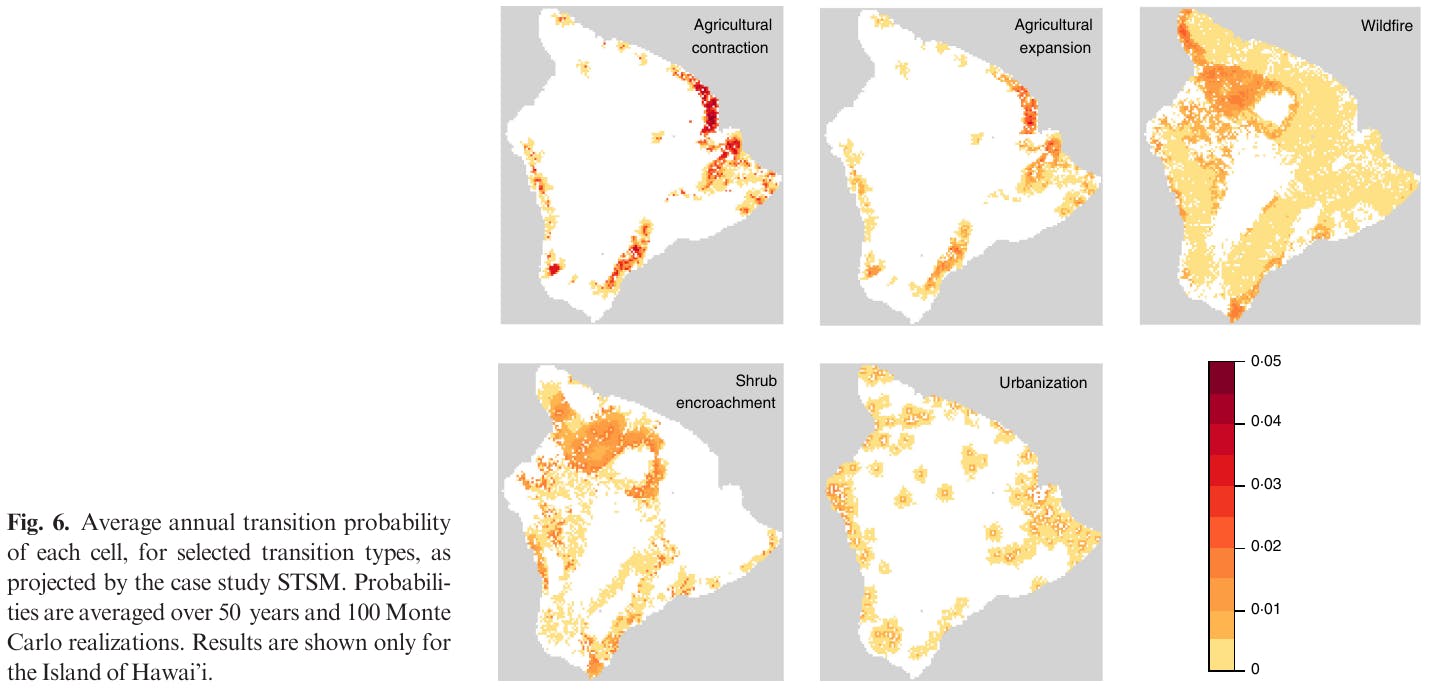
With STSMs, there are two basic forms of model output,

1. Transition output, which records when and where transitions occur
2. State output, which records the state type, age and TST

The model provides information on both forms of output for each cell, time-step and realization.

These outputs can be summarized in various ways - as time series of the area,

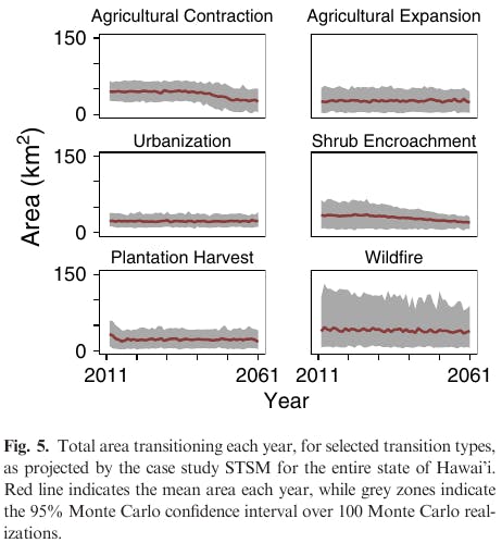
Our case study provides a sample of the type of output that can be generated with STSMs; note, however that because we present only a single future scenario, the results shown here are a scenario project for LULC in Hawai'i, and not a prediction of the likely future state.

Agricultural contraction decreases beyond this point however, due to an eventual shortfall in agricultural land. In contrast, the area projected to transition due to wildfire, plantation harvest and shrub encroachment emerges as a function of the dynamic state of the landscape, as these transitions were parameterized using probabilities.

The variability for other transitions, however, is likely underestimated given the limited historical data used to characterize their future variability.

Discussion

A key feature of STSMs is their combination of simplicity and generality; while STSMs are rooted in the intuitive principles of Markov Chains, they have important adaptations that make them applicable to a wide range of landscape management questions.

A second key feature is their explicit representation of uncertainty, an important consideration for most modeling applications.

The projections for states and transitions are expressed as distributions, rather than simply mean values, thus incorporating, through Monte Carlo simulations, the combined uncertainties of multiple model inputs.

While several of the transition rates projected by the case study model purposefully march historical distributions, the added value of reproducing these rates in the STSM is that one then able to reflect the combined consequence of multiple model inputs, including their uncertainties, on the future projections for model outputs.

The moisture zone analysis, in particular, has large uncertainties that were not modeled, highlighting the challenges of developing STSMs using the results of analyses that themselves do not incorporate uncertainty.

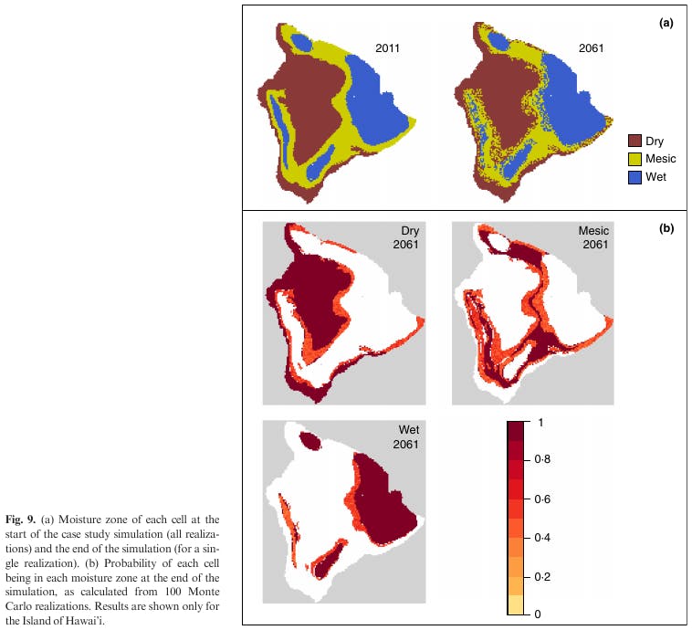
(a) Moisture zone of each cell at the start of the case study simulation (all realizations) and the end of the simulation (for a single realization) (b) Probability of each cell being in each moisture zone at the end of the simulation, as calculated from 100 Monte Carlo realizations. Results are shown only for the Island of Hawai'i

There also exist similarities between STSMs and LULC change models - like using a discrete representation of space, time, state.

For LULC, the change models divide the simulation process into two steps every timestep,

1. They calculate the total amount of change between states over one or more regions
2. Several models do this by applying a Markov chain to historical data in order to generate a matrix of transition probabilities between states

After this, the model allocates total change spatially across cells based on each cell's suitability for change.

Calculating Cell Effect

Suitability of each cell is calculated as a relative probability, which can be influenced by both external factors and neighborhood interactions.

Representing Change

1. The amount of change between states can be represented through the specification of either target areas (i.e., top-down demand), or probabilities (i.e., bottom-up conversion) for transitions.

2. The distribution of these transitions can be made to follow any spatial or temporal pattern using the STSM transition multiplier feature.

3. These multipliers can be calculated as a function of both external drivers and the state of neighboring cells.

Difference Between LULC, STSM

A major difference between STSMs and most LULC cahnge models, is the generality of the STSM method,

1. STSMs focus on those elements of landscape dynamics that are common to most applications
2. Simulating changes in the state of spatially referenced discrete random variables over time as a function of probabilistic transitions

STSM DOES NOT include specific routines for estimating transition probabilities over time, nor does it include routines for statistically fitting spatial suitability relationships or representing cell interactions.

These tasks are accomplished through the development of external models, either dynamically or a priori.

There are several benefits of this generality,

1. A single, intuitive framework can be used for a wide range of applications, including modelling both vegetation dynamics and land-use change
2. STSMs are inherently stochastic, providing a framework for capturing uncertainty throughout the modelling procss
3. STSMs provide a common framework within which alternative approaches/models can be compared

STSM Limitations

1. State-and-transition simulation models currently have some limitations. The first is that STSMs are only able to track discrete state variables. Extending the STSM framework to include continuous state variables is an area we are actively pursuing

2. With STSMs is the absence of any capability to integrate agent/individual-based models - these models have become an increasingly important approach for representing certain drivers of landscape dynamics

3. Finally, while STSMs provide the opportunity to characterize model uncertainty, through the expression of states and transitions as random variables, characterizing this uncertainty - in particular the covariance between transition probabilities - remains an important challenge

Summary

1. Forecasting models for vegetation and land use have been developed, built on spatially explicit, catered for separate applications, each different purpose and audience
2. A general framework, State-and-Transition Simulation Model (STSM), captures many of the common features, accompanied by a software called ST-Sim, built to run such models
3. STSM method divides a landscape into sets of discrete spatial units, simulating the discrete state of each cell forward as a discrete-time-inhomogenous stochastic process. Due to the spatially interacting Markov chains, there is the ability to add discrete counters such as age and time-since-transition as state variables
4. A case study of demonstrating STSM method for change of state of Hawai'i. Features for the process represented in this example include,
   • Expansion/contraction of agricultural lands
   • Urbanization
   • Wildfire
   • Shrub Environment into grassland
   • Harvest of tree plantations
5. The key outputs for the model include,
   • Projections of the future spatial and temporal distributions of LULC classes and moisture zones across the landscape
   • Over a period of 50 years
6. STSM can be applied to wide range of landscapes, including questions of both land-use change and vegetation dynamics. When combined with the ST-Sim software, STSMs offer a simple yet powerful means for developing a wide range of models of landscape dynamics